MDP Image Recognition of Symbols using YOLOv5
Achieving a high confidence score using the Roboflow pipeline

1. Introduction
This article is related to the CZ3004 Multi-Disciplinary Project (MDP) module taken in SCSE NTU. The intended audience is the Raspberry Pi team where the image recognition task will fall to. The module may change in the future but the methodology will remain the same.
I highly recommend taking CZ4042 Neural Networks & Deep Learning. For those who are not intending to take it, I added a Core Concepts section which are some concepts to get you started.
Here is the link to the Google Colab Notebook I used for training the YOLOv5 model.
Objectives


If you haven’t read the rules, the challenge is to traverse a maze of size 15 x 20 with a robot and detect 5 images using the Pi camera, noting down the image position. The symbols can differ from semester to semester. Each symbol is spread across the maze with 1 image placed in the centre that is the most difficult to reach and detect.

From what we can observe, only 1 group managed to get all 5 symbols. This speaks volumes of how difficult this task is. 8 groups did not meet the leader board criteria.
Contents

2. Core Concepts
Exam Analogy
Model training in machine learning is similar to preparing for an exam.
- Train — To prepare for an exam, we first study the lecture and tutorial materials
- Validation — To gauge if we are ready for the exam, we practice the past year papers
- Test — The exam will be the test of how well we performed in the exam
Dataset Splitting

Typically, a dataset will be split into 3 parts, train, validation and test data.
- Split dataset into train and test data
We first split the dataset into train and test images with a ratio of 80:20.
2. Split train data into train and validation data
Next, we split the training data into train and validation with a ratio of 80:20. In this step, we use the validation data to perform hyperparameter tuning.
3. Evaluate test data
Lastly, we combine the train and validation data and use it to evaluate the test data.
Split ratios may be different (75:25 or 90:10) based on dataset size.
Metrics
One of the popular metrics used to evaluate object detection models is the mAP@[.5:.95] which stands for mean average AP for IoU from 0.5 to 0.95 with a step size of 0.05 for X number of classes.
I won’t go too deep into the explanation of the metric! You can find a clear explanation of it below.
In short, the mAP@[.5:.95] score is an all-in-one metric for evaluating object detection models. It ranges from 0 to 1. The higher your mAP@[.5:.95] score, the better your model performance.
Hyperparameter Tuning
Hyperparameter tuning is the problem of choosing a set of optimal hyperparameters for a learning algorithm. There are 3 hyperparameters that have a significant impact on the model’s performance and training time.
- Learning Rate
- Batch Size
- Epochs

Learning rate is the most important hyperparameter to tune.
Comparing it to the exam analogy, it is how fast you are reading through your materials. Reducing the learning rate will mean slowing down your revision to absorb the content better. Typical learning rate values are 1e-2, 1e-3, 1e-4, 3e-4. I typically start with 1e-3 or 3e-4. The value is then halved or doubled depending on the model’s performance.
Epochs influences the training time of a model.
Comparing it to the exam analogy, it is the no. of study sessions. Reducing the no. of epochs means lesser training. The typical value I use is between 10–25, after which model performance starts to increase marginally. For initial debugging and testing, I recommend setting the value to 5.
Batch size has a significant impact on the model’s performance and training time.
Comparing it to the exam analogy, it is the no. of chapters you are revising in each study session. Reducing the batch size will reduce the content absorbed per session. Typical batch size values are 4, 8, 16, 32. In general, the optimal batch size will be lower than 32. Setting too high of a batch size may crash the model as the RAM will be full.
3. Overview of Image Recognition Task

The image recognition task can be divided into 3 steps. Each step will roughly take about half a day except modelling which took about 1–1.5 days to perfect.
⭐️ IMPORTANT LINKS ⭐️
For modelling, the video below will guide you throughout the entire process which includes:
- Uploading image data
- Data Augmentation
- Training the YOLOv5 model
- Visualizing results
Here is the link to the Google Colab Notebook I used for training the YOLOv5 model.
4. Data Collection

For data collection, the symbol attached to the obstacle was placed 10–50 cm away from the robot. We then used the Raspberry Pi to capture a stream via the picamera for 10 seconds with a display resolution of 640 x 360 px (16:9 aspect ratio). The robot is manually shifted in a clockwise direction to capture all possible angles. Next, the individual frames are extracted and saved as .jpeg files. The process is then repeated for all 15 symbols. An example of what was taken can be seen below.
If you are wondering using the picam is mandatory, it is not. Our group used both the picam and iphone to capture the images. As long as the images are taken in the arena with similar lighting, it will not affect the model’s performance. Do capture up to 100–150 images per symbol. The more images fed into the model, the stronger the model performance.
Links: picamera guide, picamera docs
5. Data Preprocessing
After the collection of our images, the next step is to remove images that will potentially worsen our model. Below are a few examples:
Symbol not captured completely
The entire symbol is not captured in frame.

Blur images
Remove images that would make labelling difficult. Slightly blur symbols are fine to keep.

6. Data Labelling
Labelling the image dataset properly is an essential step to ensuring strong model performance. In this project, we use LabelImg to label each symbol in a bounding box and save the annotation to the YOLO format.
For tips on labelling effectively, do read this article by Joseph Nelson, CEO of Roboflow. Point 4 — creating tight bounding boxes is especially important.
7. Data Augmentation
Data augmentation artificially increases the size of the training set by generating variations of the training data. [1] This reduces overfitting and allows the model to account for lighting differences and motion shift as the robot is traversing the maze.
This step is performed on Roboflow where data augmentation is as simple as adding it before downloading the dataset.
Saturation & Brightness
Accounts for lighting differences as the robot traverses the maze.


Blur
Accounts for motion blur when the image is taken while the robot is moving.

8. Modelling
The dataset can be downloaded from Roboflow to the hosted workspace in Colab. This is done by running the cell below with the custom URL. Video demo here
# Export code snippet and paste here%cd /content!curl -L “https://app.roboflow.com/ds/REPLACE-THIS-LINK" > roboflow.zip; unzip roboflow.zip; rm roboflow.zip
If you have followed the tutorial video so far, the last step will involve running the cell below to start the training process.

!python train.py — img 512 — batch 4 — epochs 50 — data ‘../data.yaml’ — cfg ./models/custom_yolov5s.yaml — weights ‘’ — name yolov5s_results — nosave — cacheLink: YOLOv5 Google Colab Notebook
9. Model Evaluation
Being able to visualize your model results is an important part of evaluating whether your model is training well.
Weights and Biases
In this project, we use Weights and Biases, which has been integrated with YOLOv5.
Here are some examples of what it is used for.


Before training the model, set up a new account on Weights and Biases and run the cells below to install and login to wandb on your hosted workspace in Colab.
Install wandb dependencies
%cd /content/yolov5/!pip install wandb -qr requirements.txt
Install and login to wandb
%pip install -q wandb!wandb login
10. Hyperparameter Tuning
For this project, I have limited the tuning process to changing the initial learning rate, batch size, epochs and optimizer.
Initial Learning Rate
To change the initial learning rate, navigate to data > hyp.scratch.yaml, change the value of lr0 to any value you like.
# Change the parameter value belowlr0: 0.005 # initial learning rate (SGD=1E-2, Adam=1E-3)
Batch Size / Epochs
Batch size can be changed under — batch while number of epochs can be changed under — epochs before running train.py.
!python train.py — img 512 — batch 4 — epochs 50 — data ‘../data.yaml’ — cfg ./models/custom_yolov5s.yaml — weights ‘’ — name yolov5s_results — nosave — cacheOptimizer
I tried using Adam optimizer but the results were not ideal for this dataset. It would be best to stick to SGD. You can read the comments by the creator of YOLOv5 here on why.
11. Results Discussion
Here are the results of the best performing model sorted by the highest mAP_0.5:0.95 score.
Table of Results

From what we can observe, the second best performing model was completed in 26 minutes and gave a pretty high score of 0.8921. The best performing model hit 0.9153.
Visualizing the best 4 models

From the graph above, we can observe that after tuning 15_classes-v1 by reducing the number of epochs, lowering the learning rate, the results improved by around 6% in 15_classes-v2-bestv1. There are also lesser amount of fluctuations as compared to the other runs.
Some runs have lesser number of epochs as the mAP score was tapering off earlier than other runs so the training was stopped midway.
After completing the training, the model weights will be stored as a .pt file where you can run detect.py on a set of images to generate the predicted label with the bounding box on the image.
!python detect.py — weights runs/train/yolov5s_results/weights/best.pt — img 416 — conf 0.4 — source ../test/imagesWe then proceeded to test the results on 2 test datasets. The images were ran using the detect.py file and images with the bounding boxes were stacked together as a video.
First Test Dataset
The first dataset comprised of 340 images and 6 symbols that were taken in a different lighting, angle and distance to test the model’s robustness.
Second Test Dataset
The second dataset (120 images) was manually selected within the dataset used where 8 images are selected for each symbol.
12. FAQs
How many images do I need to collect?
We collected about 137 images per symbol which totals to 2042 images before data augmentation.
Is the Tensorflow Object Detection API zoo worth using instead of YOLOv5?
I would recommend not. In my initial testing, I trained ssd+mobilenetv2 and EfficientDet D0 models from TFOD API but both are not as fast and accurate like YOLOv5. Additionally, the TFOD environment takes longer to setup.

What is the recommended image size?
When training the model, I set it as 512x512. When detecting images, I set it as 416x416. There is no hard and fast rule.
What is the average speed of detection using CPU/GPU?
On my laptop, it was around 0.5s. On the RTX 2080 GPU, it was around 0.01s or lesser.
My model keeps crashing on Google Colab? Why?
Once you hit the RAM limit on Colab, the model will crash. You can either set a lower batch size or get Google Colab Pro which offers a higher RAM.
How do I integrate image detection with RPi?
We adapted the code from Elelightning’s repository by using the imagezmq library to send images from RPi to the PC for detection of images.

What are some tips to improve the model performance?
The quality and quantity of the training data matters a lot. The more images you are able to supply to your model, the better your model is able to generalize and predict accurately. This can be done by performing data augmentation and increasing the image size (tradeoff is slower training).
13. Conclusion

The Multi-disciplinary project is one of the toughest mods in SCSE NTU. The amount of time I spent on this module far exceeds any module I took in SCSE (except FYP). There are just so many tasks to do aside from image recognition for the RPi team. I hope this article will save some time in figuring out how to perform image recognition of symbols. Hang in there!
14. References & Links
[1] Géron, A., 2019. Hands-On Machine Learning with Scikit-Learn, Keras, and TensorFlow, 2nd Edition. 2nd ed. O’Reilly Media, Inc., pp.450–451.